PANIC! The sky is falling! Okay, not exactly, but LSST is going to have a huge impact on NEO follow-up and it's essential that we prepare strategies for mitigating this impact before first light. Let's talk about why...
“LSST will increase the number of potential near-Earth objects identified each night by 100-1000x, and decrease the purity of those submissions by at least a factor of 10
Quick preface: On the right you'll find a table of contents so that you can hop around between topics and as you scroll the progress bar will let you know how far through you are. Throughout this page, I'll highlight any concepts that may be unfamiliar like this and then if you hover over them you can see a more detailed explanation. And before I go on, it's important to point out that this paper was very much a group effort and I'm very thankful to my wonderful co-authors who were very patient with helping me in my foray into solar system science: Mario Jurić, Peter Joachim, Sam Cornwall, Joachim Moeyens, Siefried Eggl.
Setting the Scene
Let's take a step back for a moment and cover some basic background information. First, let's talk about the stars of this production: NEOs 🪨. Near-Earth objects are defined as asteroids and comets that have a perihelion distance (its closest distance to the Sun) less than 1.3 times the distance from the Earth to the Sun. These objects are important for a variety of reasons from astrobiology to rare material mining, but perhaps most important is the potential threat they pose to Earth. To put it simply, we do not want the end up like the dinosaurs.
For these reasons it is essential that we catalogue all NEOs and calculate their orbits in order to identify any that could be dangerous for Earth. NEO follow-up is important for this task, since follow-up observations are often the best way to full constrain and orbit and confirm a potential detection from something like LSST. Currently, every night a list of potential NEOs are posted to
the NEOCP, the Near-Earth Object Confirmation Page for the follow-up network to observe. This list displays around two dozen objects per night at the moment...but that's all going to change when the fire nation attacks LSST comes online.
The Rubin Observatory Legacy Survey of Space and Time (LSST) is going to rapidly identify solar system objects from its first night of observations. Due to its ability to see fainter objects that current surveys, this will shed a new light on previously elusive solar system objects. Before this project we suspected this could have dire implications for NEO follow-up but now we have quantified this issue.
Simulating NEO follow-up during LSST
Hopefully you're now convinced it is a good idea to keep track of all of these objects! Our job at this point was to simulate how LSST will affect NEO follow-up and for that we essentially need three things:
- A simulated population of solar system objects
- A predicted schedule of where LSST will observe on each night for its 10 years
- A method for scoring each potential object to decided whether it warrants follow-up
The first step is relatively simple since catalogues of these objects already exist, in particular we use the Simulated Solar System Catalogue. We did additionally improve on this catalogue by accounting for prior known objects and created a hybrid catalogue, but I'll talk about that in a separate post.
For the predicted schedule and observations we know the baseline survey strategy plan for LSST, which outlines which areas of the sky it will observe and for how long. We used a simulator that follows this strategy but also includes predictions for the fraction of downtime and bad weather that could affect things as well. All in all these simulated observations of the solar system span over 10 years and 50 million observations!
“These simulated observations of the solar system span over 10 years and 50 million observations!
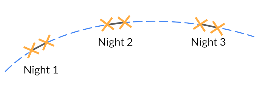
Finally, to talk about scoring potential NEOs we first need to briefly talk about observations and tracklets. Observations of solar system objects are general formed out of a series of "tracklets", which consist of at least 2 observations within a short period of time. The motion over these short periods of time is generally linear and it is easier to associate the two observations with one another. You can then connect these tracklets over time and fit an orbit to their motion (this is referred to as "linking"). Check out the digram to see an example of this where we get 3 successive nights of observations.
In reality, there are uncertainties on observations and so multiple orbits can fit the same tracklet. The scoring of these tracklets are potential
NEOs is simply done as a fraction of the orbits that correspond to an NEO orbit (which remember from above just means a closest approach to the sun of 1.3 au). This calculation is done using a code called digest2.
The impact of LSST using current criteria
Okay so now putting that all together, we have a series of mock observations of simulated solar system objects, each of which is assigned an NEO score from 0 to 100. The current threshold for submission to the NEOCP is a score of 65 and so, using thism we calculated, the number of objects that would be submitted to the NEOCP in the first year of LSST using current criteria.
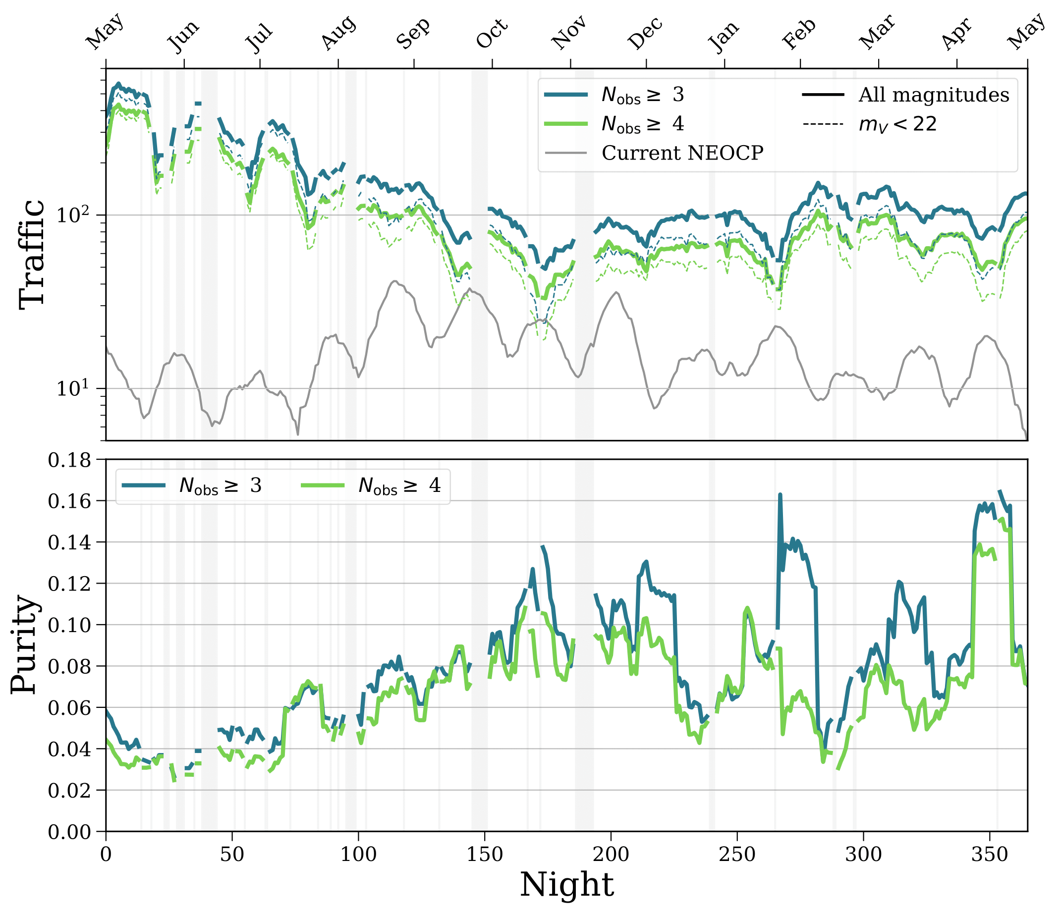
There's a lot of information in this plot so let's walk through it in detail. The top panel shows the traffic of the NEOCP, which means the total number of objects that will be submitted to the NEOCP according to current criteria. The bottom panel shows the purity, which means the fraction of the submitted objects that are actually NEOs. Each of these quantities are plotted over the first year of LSST and for a variety of required number of observations. For example, this means that the $N_{\rm obs} = 3$ line means we only include that tracklets that have at least 3 observations.
From the top panel we see that the traffic could increase to as much as 50,000 objects in a single night and the purity could go as low as 0.5%. Remember that the current numbers are around two dozen objects with a purity of around 25%. The impact of LSST is HUGE, even when requiring a large number of observations of each tracklet 😨
In case you're wondering about the general trends: the long period increase and decrease is seasonal and is due to the ecliptic plane (where MBAs reside) moving low and being observed more at certain times of year. The shorter term changes are due to the moon, you'll note there are dips in purity around every 30 days!
What about the best case scenario?
Well, that's not good for NEO follow-up! 😱 Let's imagine the best case scenario in which we can fully predict the future, would things be better? LSST can confirm many NEOs without any help from the follow-up community, so if we knew beforehand which objects would get re-observed enough by LSST then we could skip sending them to the NEOCP.
In this scenario, the traffic can still get as high as 200 objects on a single night but for the majority of the year it should still be in the current range that the NEOCP expects. The average purity is around 25% which is approximately what you find on the NEOCP currently. So this is great news!
Now the simple question is: how can we achieve or approximate this best case scenario without consulting an oracle? Time to think about some mitigation strategies!
Predicting the future to mitigate LSST's impact on NEO follow-up
We've just said that if we could predict whether LSST will perform self-follow-up on objects then we'd be able to mitigate LSST's impact. This drove us to create an algorithm that attempts to do exactly that!
For an object to be constrained by LSST it requires at least 2 observations per night, on 3 nights, in a 15 night window. (So we our miraculous foresight only needs to reach about two weeks into the future 😉). Given these requirements, we need to answer two questions
- Where will LSST point over the next two weeks?
- What is the location and brightness of the object during each exposure?
For predicting LSST's future pointings we use the rubin_sim python package to get an optimistic future schedule (optimistic because it doesn't account for unscheduled downtime due to things like bad weather). In reality one may able to adapt this algorithm to account for the fact that we'll have some short term weather forecast and increase its accuracy but we decided to make a conservative estimate.
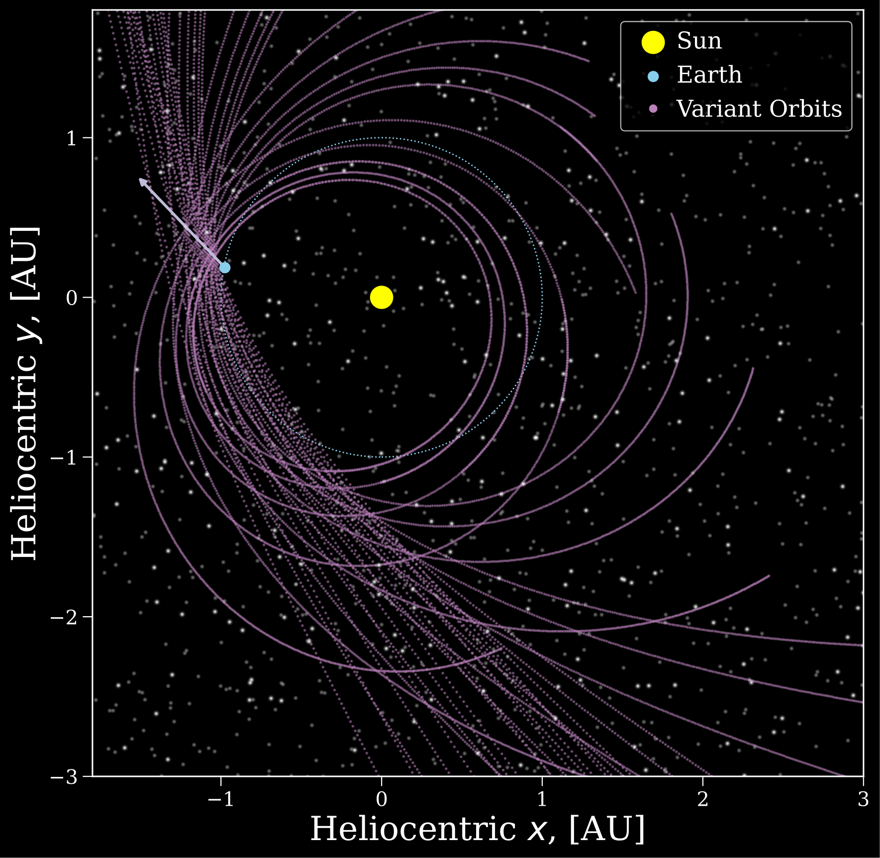
Predicting the location and brightness of the object over time requires a well constrained orbit. The problem is that, from our observations, we only constrain the on-sky position and motion, but we don't know the distance to the object or the speed at which it is moving towards or away from us. Therefore, there are many possible orbits that could fit a given observation. Check out the plot to the right that I made to illustrate this point.
You can see that given a single set of observations from Earth (in the direction of the arrow), you can get a very different orbit. To account for this we create a grid of potential orbits based on the distance and speed it is moving towards or away from us (restricted to ranges that are reasonable for an NEO).
For each of those orbits we compute its position and brightness over the course of the next two weeks using OpenOrb. From this point it is a simple matter of checking for each orbit whether it is observed at least twice on 3 nights in this window. We assign the probability of self-follow-up as a simple fraction of these orbits that achieve self-follow-up.
How effective are we at predicting the future?
So how did we do? We find that we are able to accurately predict whether an object requires external follow-up 74% of the time on average! In other words, we are able to predict the future for around 3 of every 4 objects. This has important implications for what LSST will send to the NEOCP.
Using a threshold of $p = 0.7$ for submitting an object to the NEOCP, we find that our algorithm reduces the average nightly traffic of the NEOCP back to around 200 objects per night, very close to the best case scenario! However, only around 5% of these objects turn out to be actual NEOs. Let's talk more about why this is the case and what we can do about it in the last section.
“Our algorithm reduces the nightly traffic of the NEOCP back to reasonable levels, but still results in low purity due to the MBA background
Discussion
We've shown how our new algorithm could really improve the situation but there is still the problem of purity of submissions. The main cause for the lack purity is the large background of MBAs. This isn't a problem currently as all of the brighter MBAs have been identified, however LSST will probe to much fainter depths and so there is an immense volume of undiscovered MBAs that will be observed. Hope is not lost though! There are a couple of different approaches for reducing the effect of this background that we can consider.
Improving how we score potential NEOs
The current way that we score potential NEOs only considers the 6 orbital elements but there are several other indicators of whether an object is an NEO. Some of the ones that we could consider are:
None of these factors will necessarily separate NEOs from MBAs alone, but one can imagine combining them together into an overall score. For example, if you found an object at a high ecliptic latitude, moving further from the ecliptic and it was faint and rapidly tumbling, you'd probably think it much more likely that it was an NEO!
Delaying follow-up from LSST
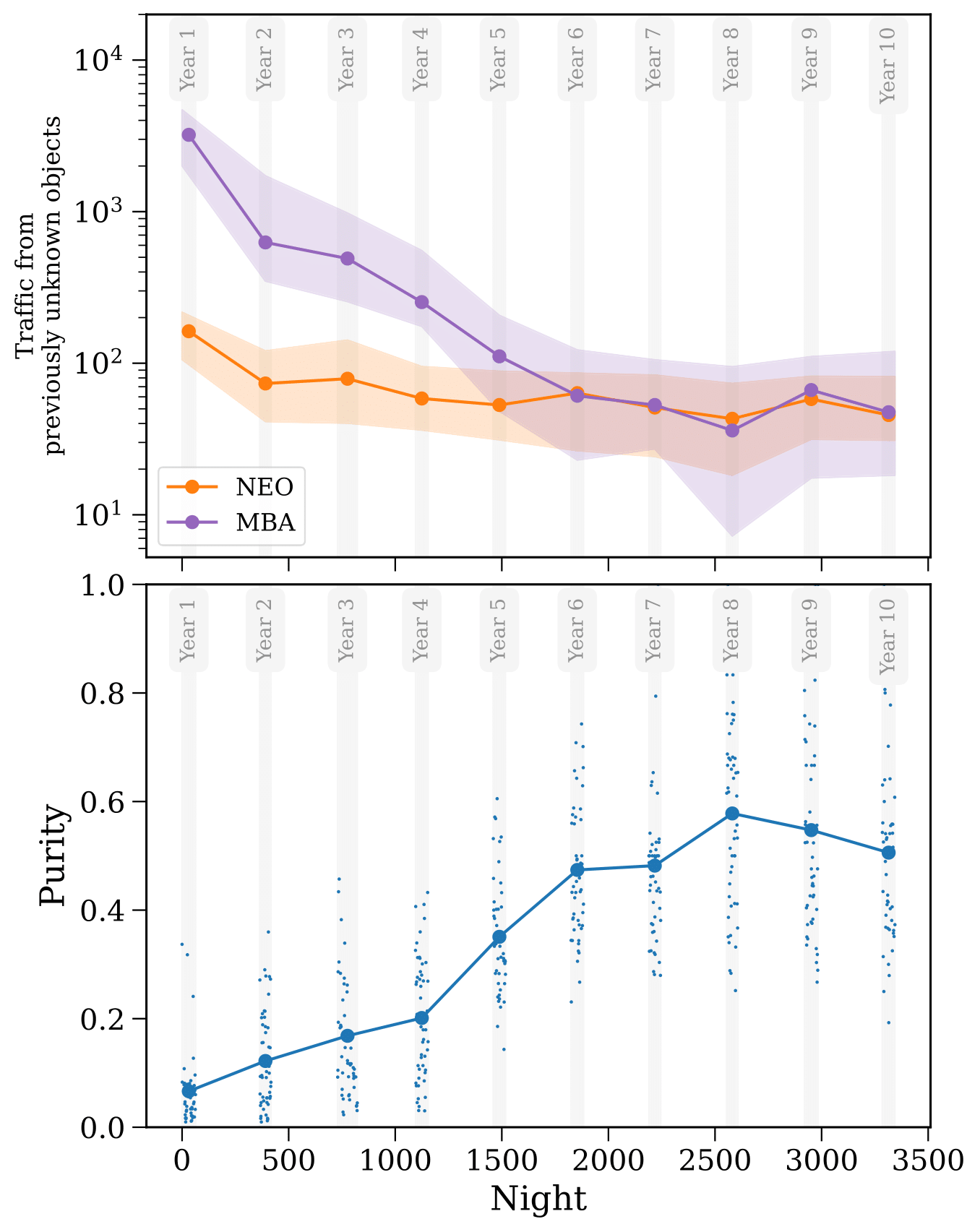
As we talked about above, the main issue is that LSST will discover a plethora of previously unknown faint MBAs and these are the unfortunate background against which we are searching for NEOs. It is expected that after the first year of LSST that 85% of MBAs will be identified. One could therefore imagine that waiting until this first year was complete would make follow-up much easier.
We tested whether delaying would have any effect and you can see the results in the plot to the right. The top panel shows how the traffic from previously unknown sources changes over the course of the 10 years (we only compute it for the first 50 nights in each year that have observations). Note the log scale, MBAs decrease drastically over the first few years before aligning with the constant steady rate from NEOs which doesn't change significantly over the entire survey.
The implications of this can be seen in the second panel, where we see the average nightly purity strongly increase as the survey progress and the remaining MBAs are identified.
We therefore recommend that general NEO follow-up from LSST not be attempted for at least the first year of LSST. However, this doesn't mean that we need to ignore every object that is identified as a potential NEO by LSST. Instead we can just place a conservative cut on the observed objects to ensure that we maintain a reasonable traffic and purity.
We explore that in one last plot to see how varying the minimum ecliptic latitude can affect the average nightly traffic and purity. If you're interested then go ahead and try out an interactive version of this plot using the button below.
Try an interactive version of the plotConclusions
I hope you enjoyed learning about this project! Click on each of the buttons below to read each of our main conclusions. Please feel free to reach out if you have any questions or would like to discuss this :)