Most current predictions for the Rubin Observatory's Legacy Survey of Space and Time use fully synthetic solar system catalogues. These do not account for the fact that we've already detected a lot of objects in the solar system. This could have some pretty important consequences - let's talk about it!
What's the problem?
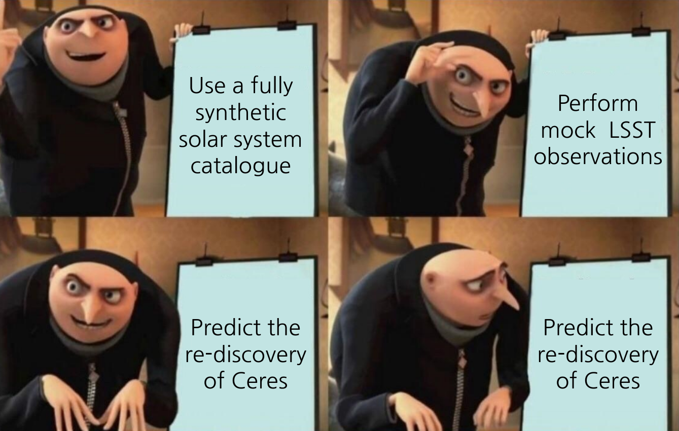
I often think that the problem with using fully synthetic catalogues is best explained by Gru (see right). As our favourite supervillain puts it, in rather extreme terms, using a fully synthetic solar system catalogue for making simulations can mean that your predictions include objects that we have known for decades.
In reality we of course would not actually predict the re-discovery of Ceres, but we would predict the discovery of a subpopulation of large/bright objects that have actually already been found in the solar system. This not only skews predictions but could also have more pragmatic consequences that we are overestimating the rate at which LSST will detect new objects.
Ideally, what we need is a full catalogue of solar system objects that has a flag for each object for whether it has already been detected. Enter: the hybrid catalogue!
Combining real and simulated catalogues
The hybrid catalogue solves this problem by combining a simulated catalogue with real data. The simulated catalogue that we use is the Synthetic Solar System Model, more commonly referred to as S3M, from Grav+2011. This catalogue contains a variety of objects including near-Earth objects, main belt asteroids, Jupiter Trojans and comets. It isn't limited by what we can/have observed and is intended to approximate the distribution of all solar system objects.
For the real data, we use the Minor Planet Center's Orbit Database (MPCORB), which contains the details for every small solar system object that has been detected to date. This catalogue is updated frequently as new objects are detected.
The idea is that we can merge these two catalogues by replacing synthetic solar objects with real analogues. The difficult part of this is finding "similar" objects between the two catalogues. We can't simply randomly replace synthetic objects with real ones since we don't want to change the underlying distributions in the simulated catalogue. This means we have to be a little smarter about how we merge them.
How does the algorithm work in practice?
As we said above, the key is to replace similar objects. We use 7 parameters to define similarity between objects: position ($x, y, z$), velocity ($v_x, v_y, v_z$) and absolute magnitude ($H$, sort of a proxy for size). To start, we separate the catalogues into bins of absolute magnitude and then for each real object in that bin:
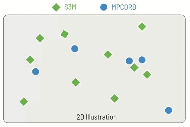
- Find the nearest 100 simulated objects (in terms of position) to the real object that are within 0.1 AU
- Select the subset of those nearest objects that have not already been assigned
- If no objects remain, inject the real object directly into the hybrid catalogue, otherwise assign the object with the closest velocity to be replaced by this real object
The reason that this is tricky is the "that have no already been assigned part" - which means that you can't do this operation efficiently in parallel since each result depends on the earlier results. We speed this up by using a K-D Tree to find the nearest objects.
I've made an example of how this might work in just two dimensions (instead of 7) in a small animation. You can see that for each real objects (blue circle), we identify the closest simulated object (green diamond). For the fourth real object it becomes more difficult, since the closest simulated object has already assigned and so we must choose the second closest simulated object. Finally, for the fifth real object, it is so far from any of the simulated objects that we do not perform a replacement but instead inject it directly into the hybrid catalogue.
Assessing how well we combined the catalogues
So, hundreds of millions of objects and several hours on the computing cluster later, we have our hybrid catalogue! Now the question is how well we did at combining the catalogues intelligently to keep the underlying distributions unchanged.
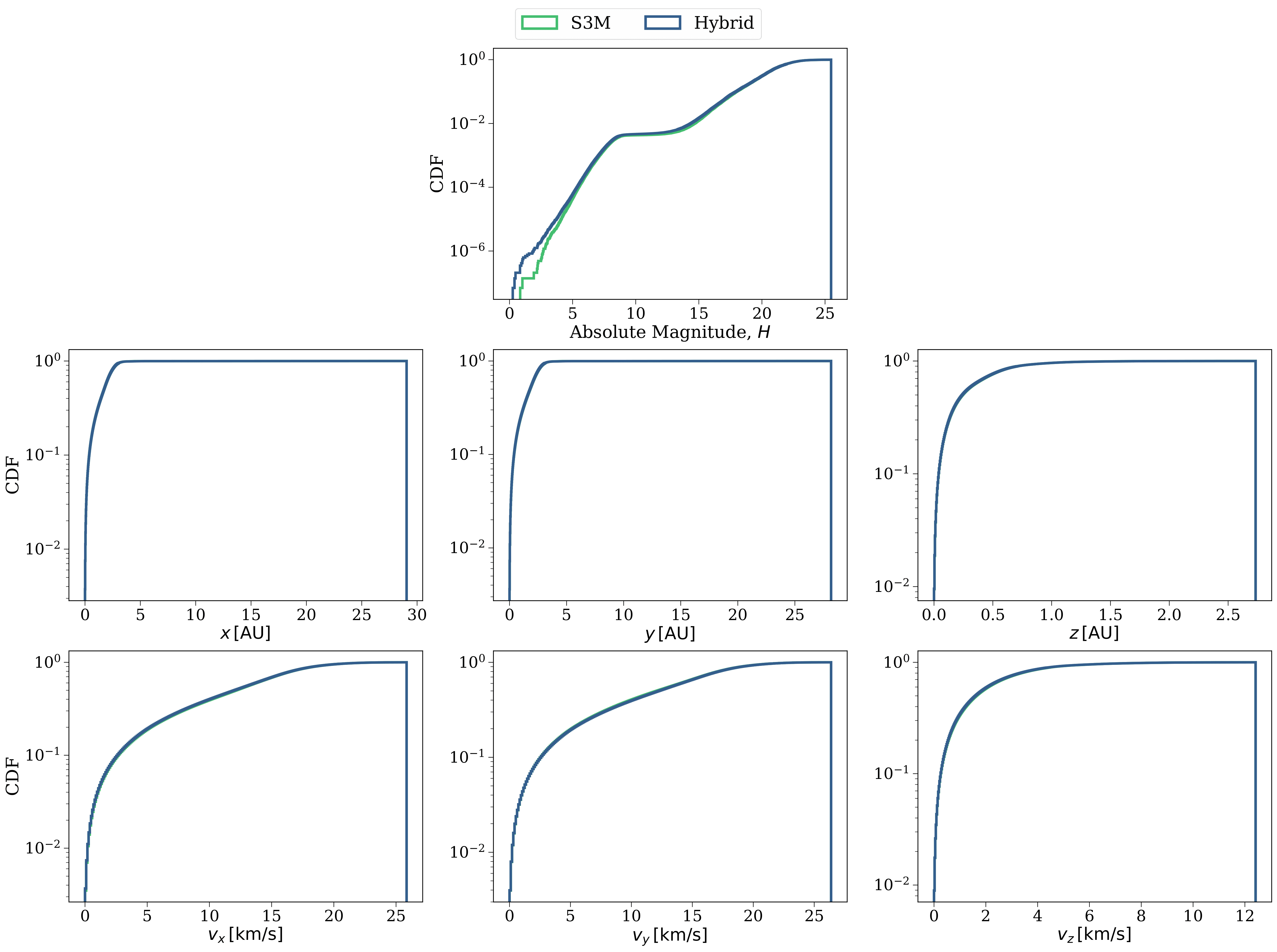
Let's first plot up the cumulative distribution functions of each of the 7 parameters that we used to determine whether two objects are similar. Check out the plot to the right, the top panel shows the absolute magnitude, the second row is the position and the third row is the velocity. In each panel we plot a green line for the synthetic S3M model and a blue line for our new hybrid catalogue. One immediate thing to note is that in most panels you can only really see one line, the two distributions align almost perfectly!
The one difference that you can see is for the smallest absolute magnitude objects. We see that the hybrid catalogue has slightly more bright (meaning large) objects than S3M. This is due to the objects that are added directly since they don't have near neighbours in our parameter space. To put it another way: we have discovered several bright objects that were not directly represented in the simulated dataset.
Okay so they look the same but let's be a little more quantitative than that. A common way to check whether two samples are drawn from the same distribution is to use a K-S Test. We find when applying this test that both catalogues are consistent with having been drawn from the same distribution. Sounds good so far!
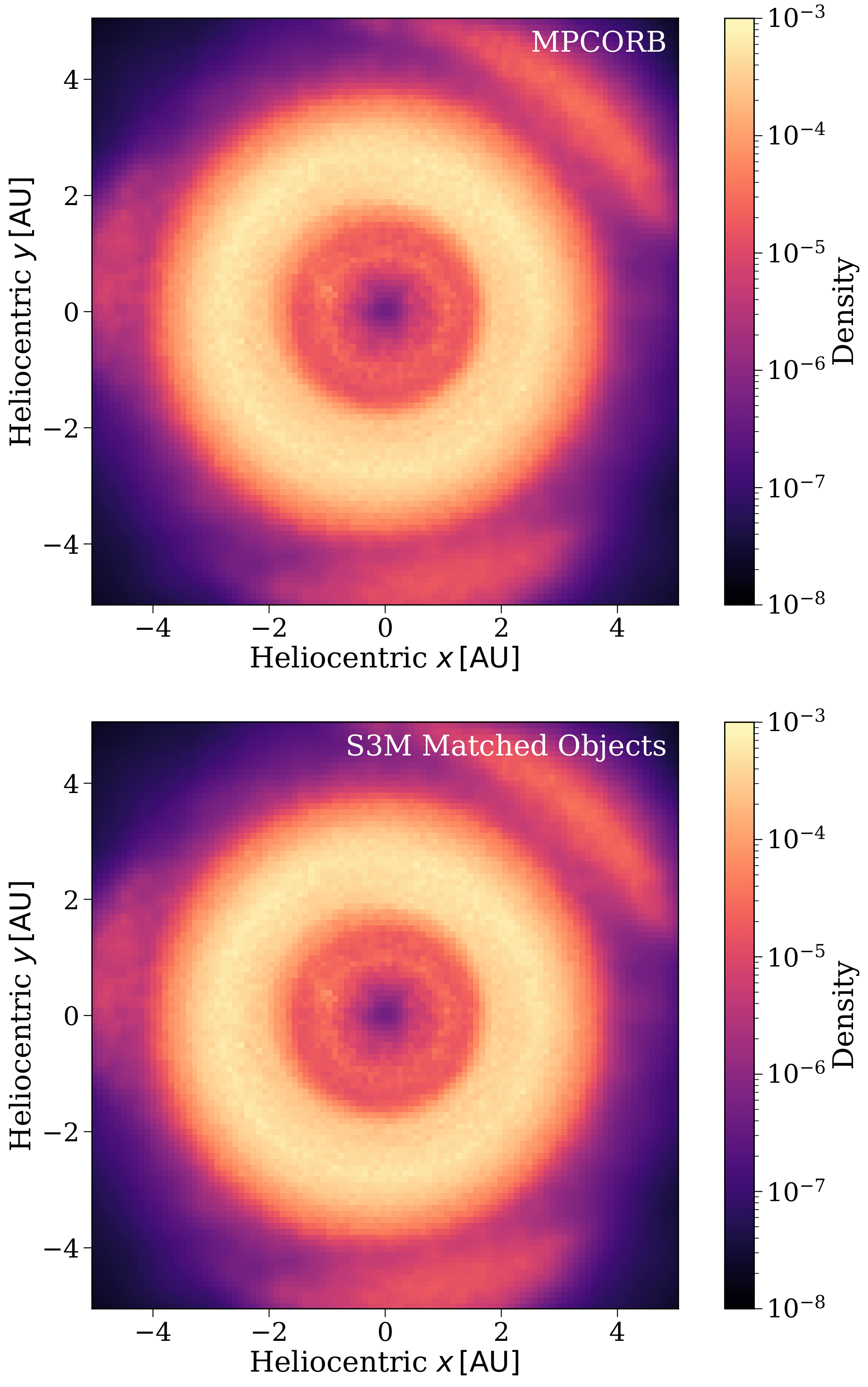
Let's do one more check just to be sure. This time I'd like you to spot the difference between the two density distributions on the left 🙃 The top panel shows a distribution for the real detections from the MPCORB database, whilst the bottom panels for the distribution of objects that our algorithm matched to be replaced by the MPCORB objects.
Each plot is showing the density distribution of objects within 5AU (5 times the distance from the Earth to the Sun) of the Sun. Brighter areas have more objects and dark regions correspond to voids. You can see a couple of fun things in these plots:
- The central thin ring around 1au are likely objects that were identified as NEOs
- The thick bright ring centred on 3au is the asteroid belt
- The regions of higher density outside the ring are the Jupiter Trojans
Now you can take a moment to stare at these two density plots and try to see some differences. Hopefully you agree with me that it's hard to find much of a difference (especially given that the colour scale is logarithmic).
Once more we can be a little more quantitative about this and check the KL Divergence of the two densities. This gives a measure of expected excess surprise from using one density distribution as a model and managing to draw the other one. A value of 0 would indicate identical densities and we find a value close to 1 which indicates extremely similar densities. Once more this indicates we did a good job!
Wrapping up
Our framework for building hybrid catalogues manages to retain the underlying distributions of synthetic catalogues, whilst also identifying which objects have already been detected. This means that we can make predictions that account for prior solar system detections.
You can try this out for yourself using the hybridcat code, available on GitHub and pip installable!