On this page, I've done my best to explain (without the cryptic jargon and any assumed background knowledge) the motivation behind, methods used and results found by my paper on detecting Galactic LISA sources with LISA. On the right you'll find a table of contents so that you can hop around between topics and as you scroll the progress bar will let you know how far through you are. Throughout this page, I'll highlight any concepts that may be unfamiliar like this and then if you hover over them you can see a more detailed explanation. And before I go on, it's important to point out that this paper was very much a group effort and I'm very thankful to my co-authors: Floor Broekgaarden, Selma de Mink, Neige Frankel, Lieke van Son and Stephen Justham.
Why investigate gravitational waves?
So before we get into the paper, let's take a step back and consider why it is interesting to investigate gravitational waves. We've already got a bunch of telescopes that can observe pretty much anything in the electromagnetic spectrum, so why bother? Well, what if what you're observing is behind a giant dust cloud, or doesn't emit any light? In this case, gravitational waves could shed some light (pun intended) on a problem that would otherwise have been unobservable.
For our purposes, gravitational waves are emitted when two objects spiral around one another. This could be as simple as two dancers performing or two ice skaters holding hands and spinning around one another. Or, it could be as dramatic as two black holes spinning around one another, closer and closer until they merge. The difference is that the waves from those two black holes are significantly stronger (and so, easier to detect) than those that you're emitted with your friend on the ice rink.
It is also important to highlight that the emission of gravitational waves is what causes two objects (like two black holes) to merge. The gravitational waves carry away energy from the system and so the two objects have to get closer to one another to compensate. This process accelerates over time until the dramatic gravitational wave merger occurs.
Gravitational waves can give us access to regimes that were previously unobservable. Black holes themselves will emit no light without an accretion disc, and even then it is difficult to learn more about the objects. However, gravitational waves can be used to observe black holes directly in binary systems. The extreme gravity around black holes and neutron stars can be used to test the accuracy of general relativity as well as provide measurements on the Hubble constant, which measures the rate of expansion of the Universe. On top of all of this, black holes and neutron stars are the endpoints of massive stars and so we can use them to learn more about how these types of stars evolve.
Why use LISA to study double compact objects?
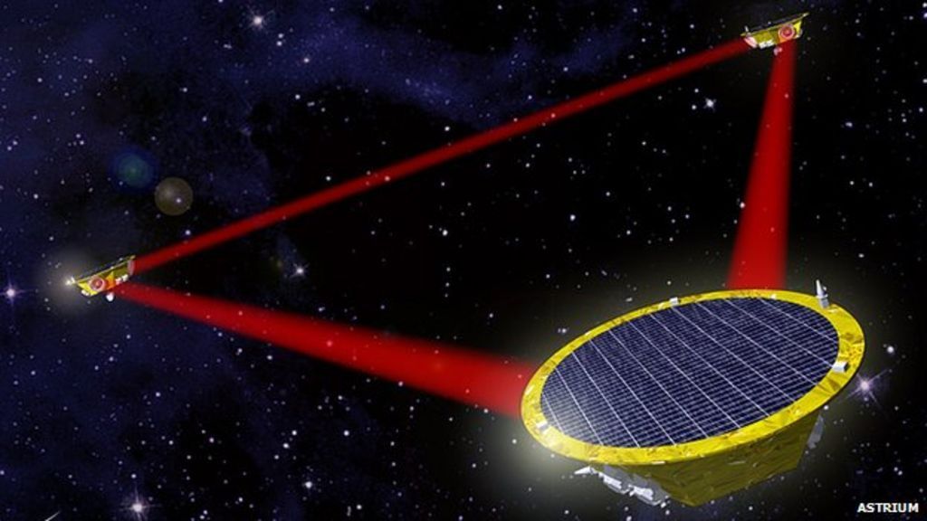
So hopefully you now see why gravitational waves are interesting to study, let's talk more about why LISA is useful. LISA is a space-based gravitational wave detector that will consist of three satellites that will orbit the sun (following the path of the Earth). The image shows an artist's impression of what it will look like. As you may be aware, we already have several operational gravitational wave detectors. LIGO, Virgo and Kagra have already detected several gravitational wave mergers, so you may ask, why do we need LISA?
LISA will observe gravitational waves at a lower frequency than ground-based detectors. This means that you can observe a local (within the Milky Way) stellar-mass binary long before the emission of gravitational waves causes it to merge. These sorts of detections have a lot of potential for discovery, we could learn more about a whole array of phenomena, including r-process enrichment, kilonovae, short gamma-ray bursts and neutrinos. LISA could be used to constrain the existence the so called "lower mass gap" in the black hole mass function. Currently, we haven't detected any black holes with masses between 2 and 5 times the mass of the sun and scientists wonder if this gap is just from observational or is the result of some sort of formation process. Additionally, LISA could link gravitational wave detections to pulsars found with the Square Kilometre Array and this could be used to refine the measurements in both detectors.
Hopefully you're now as excited as me about the potential of gravitational wave detections with LISA and now we can talk about my paper and the sorts of detections that I predict LISA will have!
How did we produce our results?
In order to learn about the LISA detectable population of binary black holes (BHBHs), black hole neutron stars (BHNSs) and binary neutron stars (NSNSs), we ran several detailed computer. We took a large population of binaries, positioned them such that they resemble the Milky Way and then evolved them until present day. We then repeated this all many times to work out how uncertain our results were.
First, we need some binaries
So first, the binaries. We use simulations from Floor Broekgaarden's recent (and upcoming) papers. Floor used the population synthesis code COMPAS to produce a huge grid of over 2 billion massive binaries. This code essentially follows a series of rules that state how the luminosity and temperature of a star changes over time and also what sort of compact object the star becomes upon its death. These rules are based on very detailed stellar models, which computed the evolution of certain stars based on the equations of stellar structure. You can read more about how COMPAS works in our methods paper and also more about how the original models were computed in Hurley et al. (2000, 2002).
Floor's simulations also cover 20 different binary physics variations. This means that each simulation changes a setting in the COMPAS code to explore how the results change if we assume something different about binary physics. This is important because a lot of binary physics is still unknown and so by exploring these changes we can see how important each uncertainty is for LISA detections.
Next, we need to decide where to put them
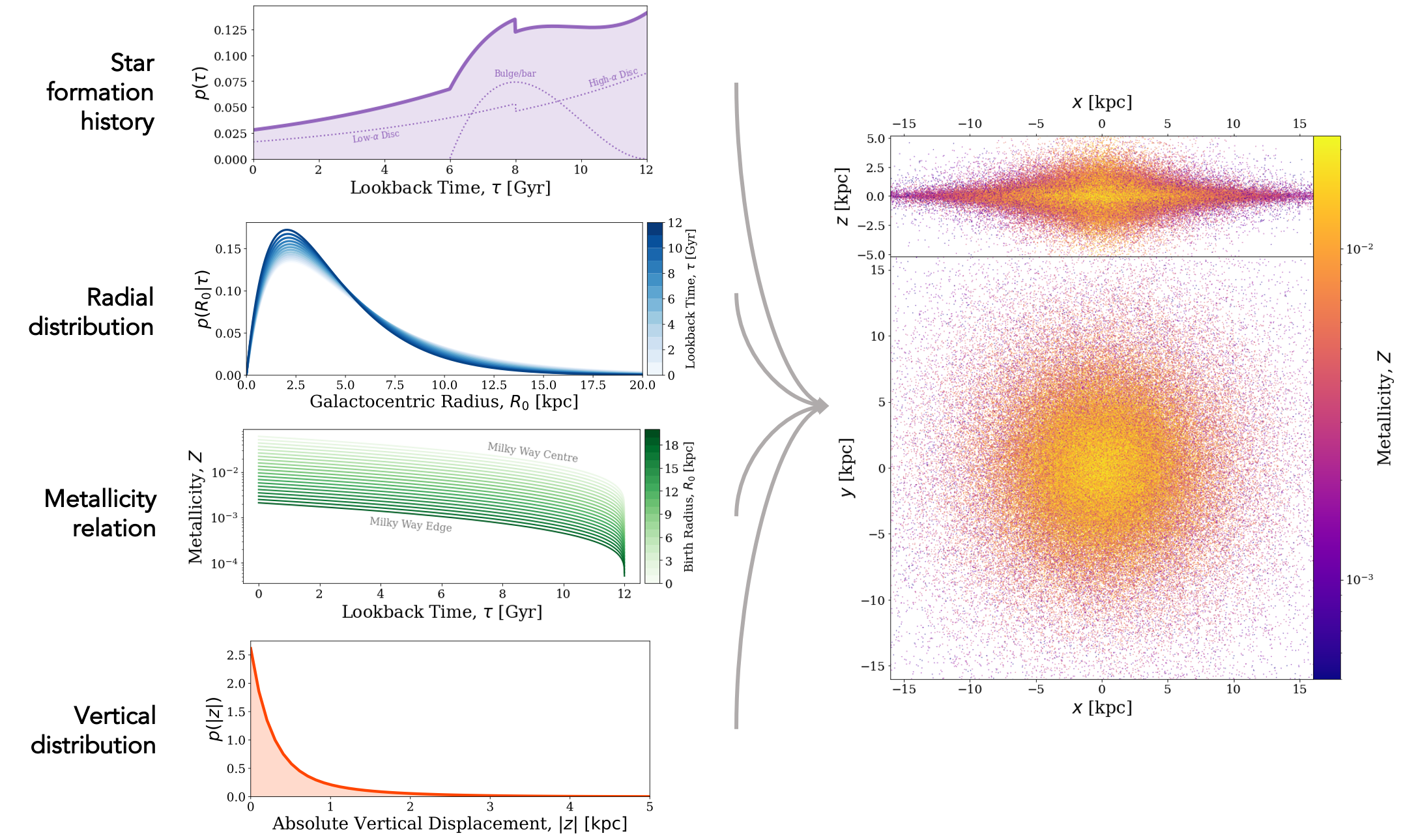
Time to build a galaxy! For this part of the paper, Neige Frankel's expertise was essential. She helped us to design a new model for the Milky Way. This model was created based on data from the APOGEE surveys. The model contains three different components: a central bulge/bar component in the centre of the galaxy, a thick disc, which contains older stars and is more vertically spread out, and a thin disc, which contains younger stars and is less vertically spread out. The distribution in terms of positions and birth times in each component is different and is shown in the figure.
Other than its more complex models for the birth times and positions, the main of this model is that it is metallicity dependent. This means that the position and birth time of a system corresponds to its metallicity. Previous studies just assumed the same metallicity for every system and this can produce misleading results.
The figure shows show the different galactic parameters are distributed. For example, the purple plot shows that most systems are formed earlier in the galaxy, whilst fewer are formed in the past 2 billion years or so. The right hand side shows an example Milky Way created using this model with both a face-on and side-on view.
And finally, we need to work out which ones turn out to be detectable
Last, we need to evolve the sources until present day and work out whether LISA could detect them. Enter
LEGWORK, a Python package that I developed with Katie Breivik with this exact purpose in mind! We use the package to evolve the sources over time and then calculate their signal-to-noise ratios in LISA. For any sources that have a signal which is 7 or more times stronger than the noise, we mark it as detectable. For more information about LEGWORK check out the release paper
on the ArXiv!
What does the detectable population look like?
Great! So now we follow the methods above to produce many different Milky Way instances and find detectable populations in each one. We repeat this for every different physics variation and also each double compact object (DCO) type (BHBHs, BHNSs and BHNSs). The result of all of this is collection of detectable sources that we can analyse to see what sort of things LISA will see. For a 4-year LISA mission, our fiducial model predicts that, on average, LISA will detect 74 BHBHs, 42 BHNSs and 8 NSNSs. And that's an important enough results for me to repeat it in a blockquote for anyone skimming through this!
“For a 4-year LISA mission, our fiducial model predicts that, on average, LISA will detect 74 BHBHs, 42 BHNSs and 8 NSNSs
Note that for this section we're just going to consider the fiducial model and we'll look more at the physics variations in a later section.
Distribution on the LISA sensitivity curve
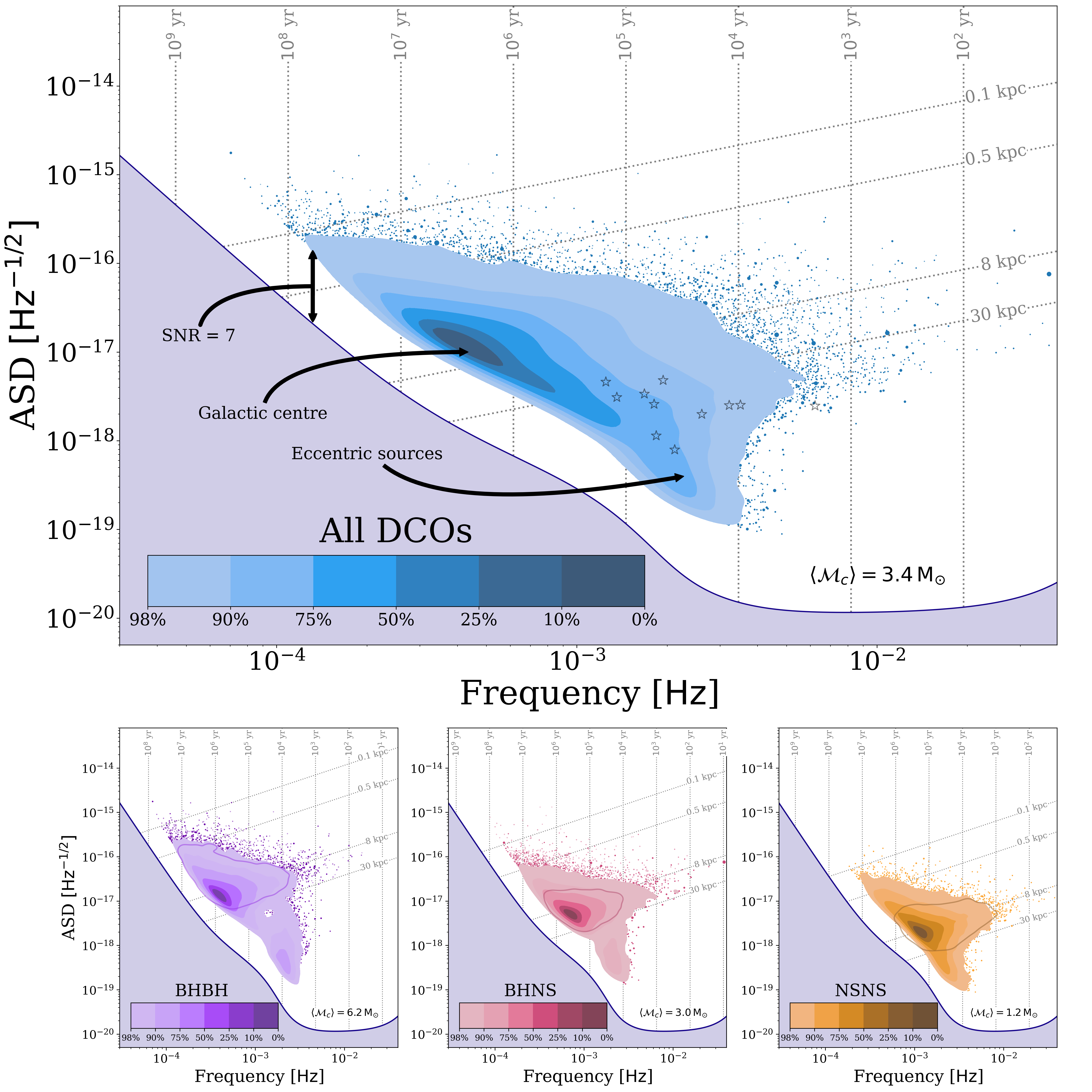
A common way of visualising a detectable population in LISA is to plot the sources on the LISA "sensitivity curve". The sensitivity curve shows how well LISA can measure signals at different frequencies. The higher the sensitivity curve at any frequency, the more difficult it is to detect a source at that frequency. For binaries, the frequency shows how quickly the two objects are orbiting one another. The higher the frequency, the faster the objects are orbiting. This means that sources on the left side of the plot are spinning slowly, whilst those on the right side are spinning quickly and getting close to merging.
Let's just focus on the top panel for now, which contains all three types of DCO together. Each source is plotted at the frequency where it emits most of its gravitational waves and its height above the sensitivity curve tells you its signal-to-noise ratio. Since there are so many sources we don't plot them individually but show a density distribution instead. The blue area shows the density distribution, where the darker the density distribution is the more systems are found in that location. The first thing we notice is that there is a gap between the sensitivity curve and the distribution, this is because we only show detectable sources and they have to be 7 times higher than the curve by definition! You can also see that the darkest part of the distribution (i.e. where most sources are detected) coincides with the line for 8kpc, which is roughly the distance to the centre of the galaxy. This makes sense since most sources are formed at the Galactic centre so it also follows that are most are detected there.
Now let's look at the lower panels. It is slightly difficult to see but, if you look closely, BHBHs are detected at lower frequencies than BHNSs and the same is true for BHNSs relative to NSNSs. You'll also see this more in the next section. Finally, in each of the panels you can see there is a sort of "offshoot" that extends lower than the rest of the distribution. We show in the paper that this is from eccentric systems and so you can possible identify them from their location in the sensitivity curve.
Properties of detectable sources
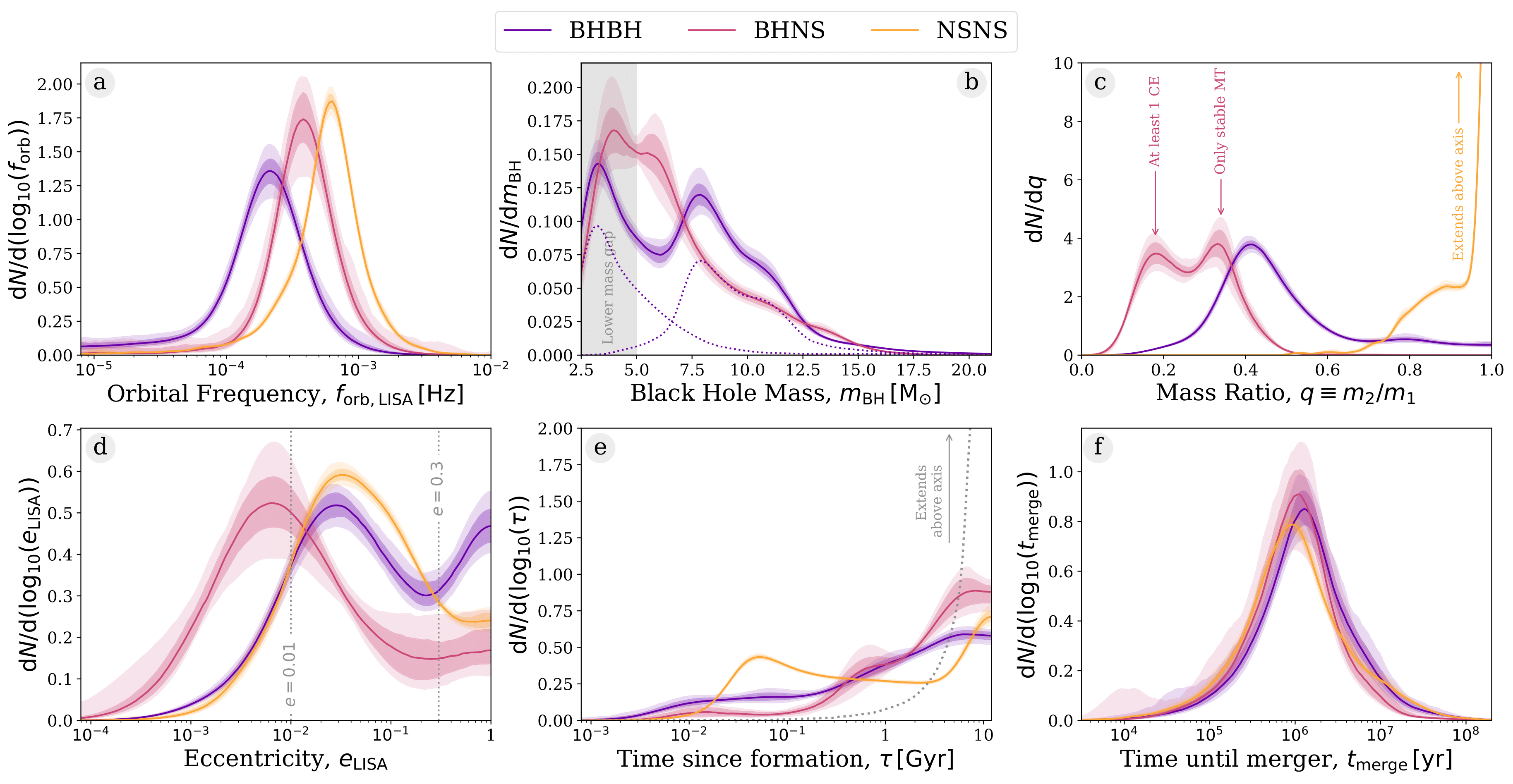
Now let's take a look at some of the different parameters of the detectable systems. The plot shows the distribution of 6 particular parameters for the fiducial model. Note that explaining the distributions that we see can be require quite a lot of background knowledge so I'm only going to describe what we see in this section and if you want to read more about why the distributions looks this way then check out Section 3.2 in the paper. Also note, that you can click on the plot to zoom in!
In each panel, there are three curves which show the distribution for a different DCO type. BHBHs are purple, BHNSs are pink and NSNSs are yellow. In the first panel (a), we see that the orbital frequency is generally most likely to be on the order of half a millihertz. Importantly, we note that BHBHs are detected at lower frequencies than BHNSs, which are in turn detected at lower frequencies than NSNSs.
In the second panel (b), we show the distribution of the black hole mass (and hence NSNSs are not in this panel). A key point from this plot is that there is a large fraction of systems detected in the "lower mass gap" and we'll discuss the importance of this later on. Another thing to notice is that the BHNS and BHBH curves has two peaks. The BHBH peaks come from the primary and secondary black holes generally having unequal masses, whilst the BHNS peaks come from having a mass ratio distribution with two peaks. This leads us nicely into the mass ratio panel.
The mass ratio panel (c), shows that the different DCO types have very different mass ratio distributions. The mass ratio tells you how the masses of two compact objects in a binary compare. A mass ratio of 1 means that their masses are equal and the lower the mass ratio, the more unequal the mass are. NSNSs have mass ratios very close to 1 usually and so we see that they are usually equal mass in our simulations. In constrast, BHBHs and especially BHNSs generally have lower mass ratios and so the two objects don't usually have equal masses. This is expected for BHNSs since black holes and neutron stars have very different masse, but this is surprising for BHBHs.
The fourth panel show the eccentricity distribution. Importantly, we find that all detectable DCOs have nonzero (and sometimes, significant) eccentricity, which can be useful for distinguishing them from other LISA sources which are often circular. BHNSs are the most circular (closest to $e = 0.0$) of the DCO types. NSNSs have the most "mildly eccentric" ($0.01 < e < 0.3$) population, whilst BHBHs have the largest highly eccentric population.
“We find that all detectable DCOs have nonzero (and sometimes, significant) eccentricity, which can be useful for distinguishing them from other LISA sources which are often circular
We show how long it has been since each DCO formed in the fifth panel (e). The grey dotted line shows the distribution of when systems were formed (no matter whether they are detectable). So we see a stark contrast between the main population (which is mostly formed at early times) and the detectable populations (which are mainly formed at relatively recent times). In the last panel (f), we show how long it would take each system to merge after being detected in LISA and you can see that each DCO type shows approximately the same distribution and that most systems will take roughly a million years to merge.
Where are detectable sources in the Milky Way?
So we've talked about what the sources are like, and where they lie in relation to the sensitivity curve, but what about something more intuitive like where they are in the Milky Way?
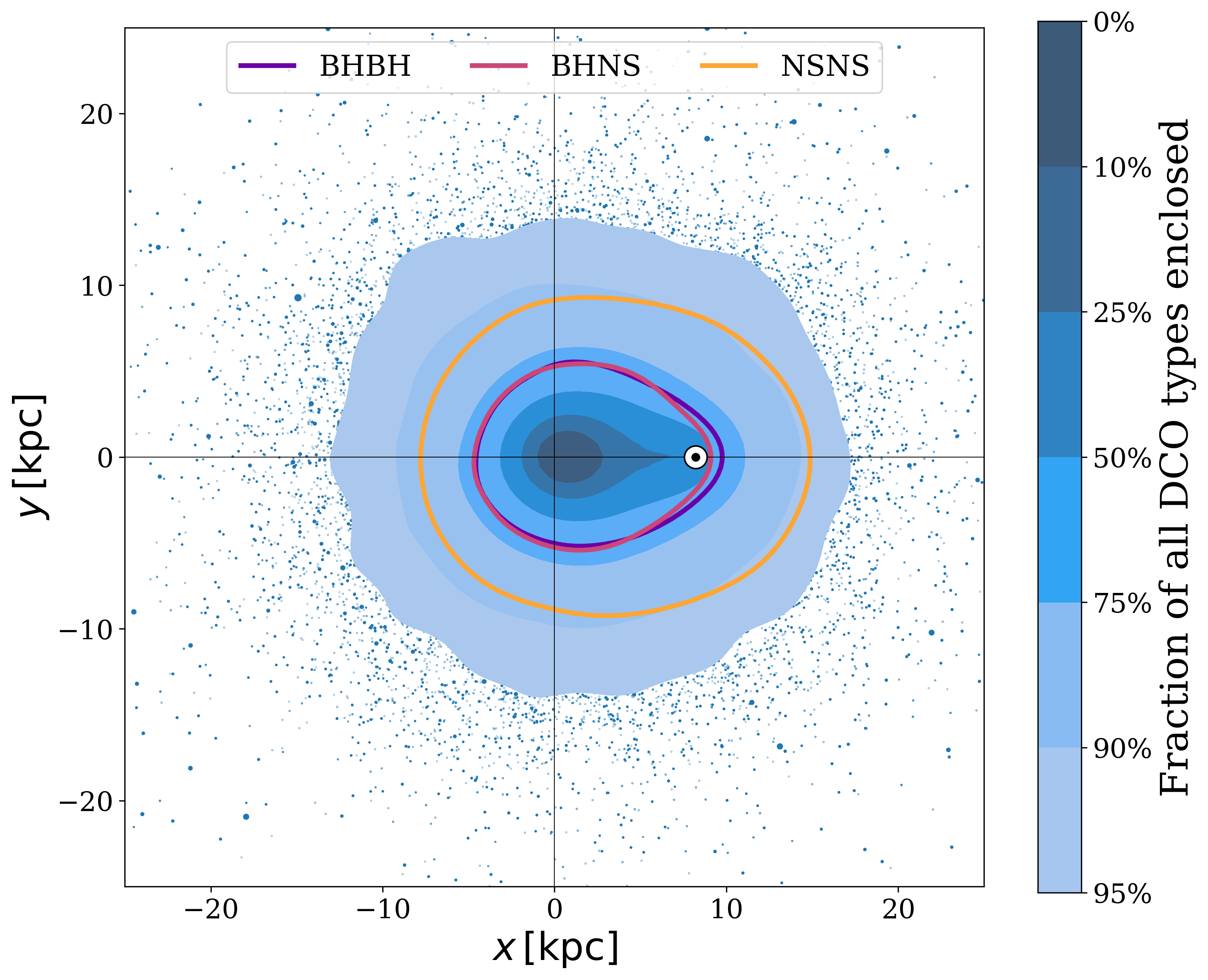
The plot shows how the detectable systems are distributed in the Milky Way with a face-on view. First some quick notes on how the plot is set up: the axes are centred on the Galactic centre, (0, 0) kpc, and I've added some black lines to guide your eye. You can also see a small circle with a dot in it, this represents the location of the solar system.
The blue density distribution (and points) show where all detectable DCO types are found. As expected the peak is in the Galactic centre, since that is where most systems are formed. There is also a slight bias where the peak is not quite in the centre and is actually slightly closer to the solar system. This is because systems that are closer to LISA are easier to detect and so we are more likely to detect them closer to us. The coloured lines show where 90% of each individual DCO type is found, where BHBHs and BHNSs are fairly similar, though NSNSs can be detected a slightly larger distances.
How well can we measure these sources?
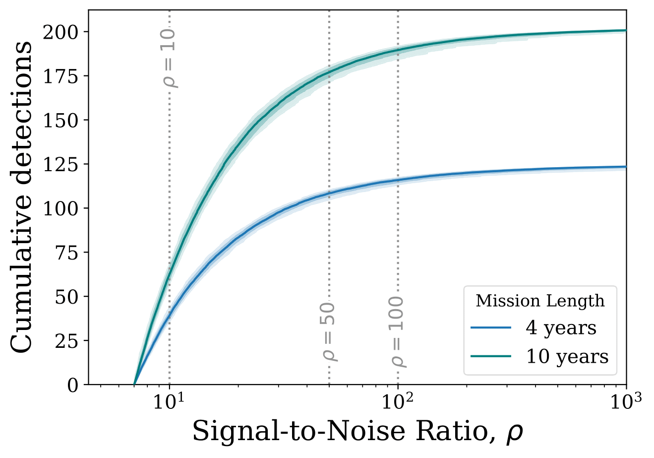
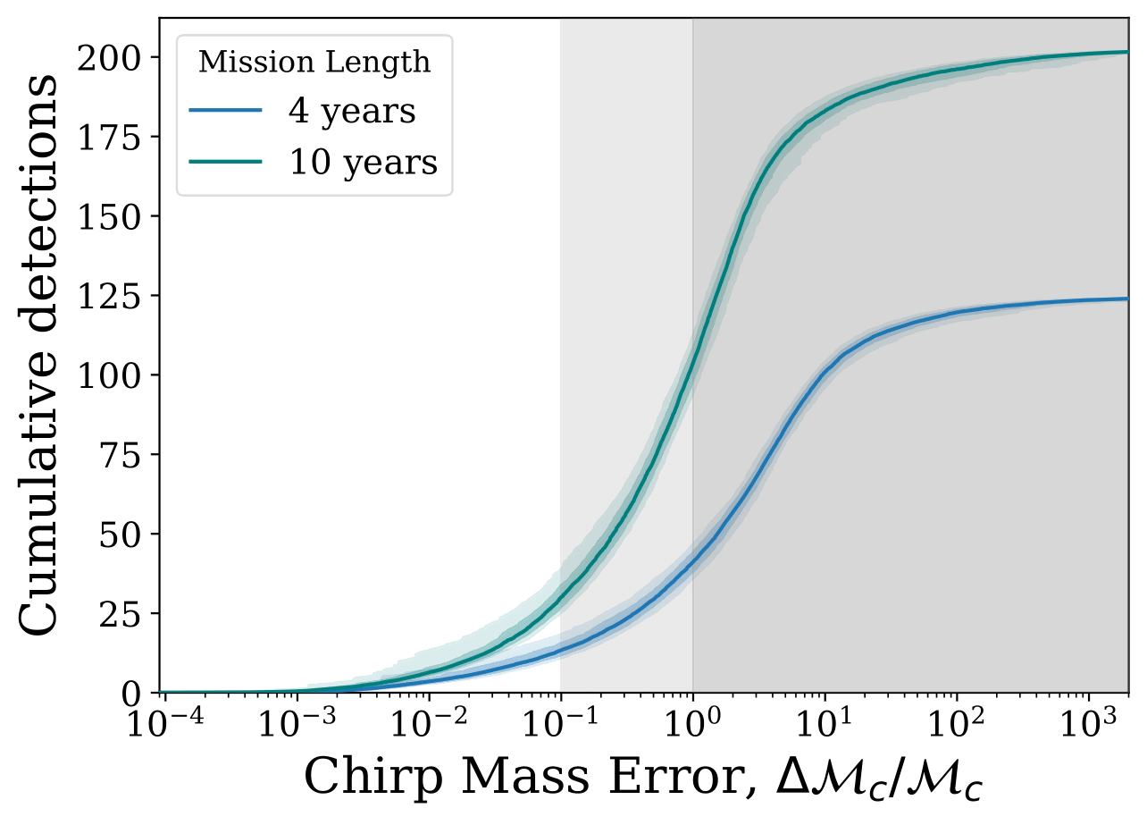
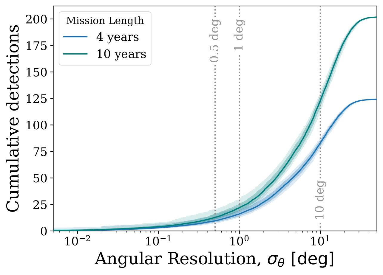
An important question to ask is how well can we measure these sources. It's all well and good that we can predict from simulations what the properties of the detectable systems, but we also need to know what LISA will actually measure. In a series of plots below, I've shown you the distribution of signal-to-noise ratios, the error on the chirp mass and the angular resolution as cumulative distributions that are scaled to the expected number of detections in our fiducial model. This means that the y-value at any given x-value tells you how many detections have that x-value or less.
The signal-to-noise ratio plot shows that many systems are detected with an SNR less than or equal to 10 and won't be very well measured. However, we also see that there are sources with very high SNRs (up to hundreds!). The second plot shows how well could measure the chirp mass, which is a quantity that combines the two masses of a binary in a certain way. The way to read this plot is that only systems out of the dark shaded regions have chirp masses that can be measured at all and only systems outside of the shaded regions can be well measured (with at most 10% errors). Finally, the last plot shows how well we can resolve a source on the sky (i.e. work out what direction it came from). To give you a useful comparison, the angular size of the moon on the sky is about half a degree. So you can see that in a 10 year mission, about 25 sources can be localised to a region that is no bigger than the size of the moon in the night sky.
How does varying our physics assumptions change the results?
So far, we have only shown results for our fiducial model, but we should also examine how altering our assumptions about binary physics could change our results. We find that, over our 20 physics variations, the expected number of detections in a 4-year LISA mission varies between approximately 30 and 370. This increases to between 50 and 550 for a 10-year mission. The variations that we consider probe some of the more uncertain areas of binary physics and we aim to investigate out the relative importance of each assumption.
“We find that, over our 20 physics variations, the expected number of detections in a 4-year LISA mission varies between approximately 30 and 370. This increases to between 50 and 550 for a 10-year mission.
Below, we show how changes these assumptions affects not only how many systems are detected by LISA, but also the properties of the detectable systems.
Effect on the number of detections
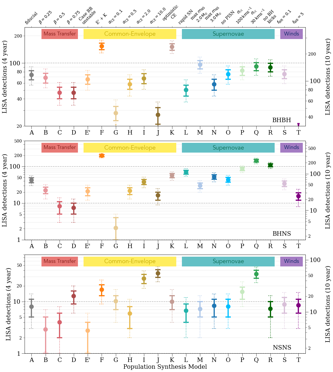
The first thing that we can investigate when changing the underlying physics assumptions is simply how many DCOs will we detect and this is exactly what the plot shows. The three panels correspond to BHBHs, BHNSs and NSNSs respectively. Each point corresponds to a model on the x-axis (from A to T), which are also labelled on the top of the plot in slightly more detail. The y-axis gives the detection rate in a 4-year mission on the left and a 10-year mission on the right. Note as well as the y-axis is a logarithmic scale not linear!
We split these variations into four main categories (show in the coloured banners): mass transfer (variations relating to how the two stars transfer mass between one another), common-envelope (variations relating to how common-envelopes are initiated and ejected), supernovae (variations related to the compact objects left behind after supernovae and the kicks that they receive) and finally stellar winds (variations in the strength of Wolf-Rayet-like winds).
In the paper we describe in detail how each variation affects the detection rate and suggest explanations for these trends. This is another part that would require a lot of background knowledge and detail to explain so I recommend that you check out Section 4.1 if you'd like to learn about why these trends appear!
“Different choices in regards to binary physics assumptions can strongly affect the predicted detection rates for LISA
However, we can still remark on the general trends. First, we can see that changing our choices for the maximum neutron star mass (models M and N), not implementing pair-instability supernovae (model O), changing our remnant mass prescription (model L), or decreasing the efficiency of Wolf-Rayet-like winds each have very little effect on the detection rate for each DCO type. However, the rest of the models can effect changes of at least a factor of two in the detection rate. These large changes therefore highlight the fact that it is important to consider these model variations since different choices in regards to binary physics assumptions can strongly affect the predicted detection rates for LISA.
Effect on the properties of detectable systems
Although it is interesting to see how the number of detections is affected by assumptions we make about binary physics, it would be a mistake to summarise these changes with a single number. It is also important to examine how the properties of detectable systems change.
However, it would be impossible (or, at least, not very pleasant for you to read) to show how every parameter of the system changes for every model variation. In the paper we focus on three in particular and I will highlight one of them here (check out Section 4.2 of the paper to see the others!).
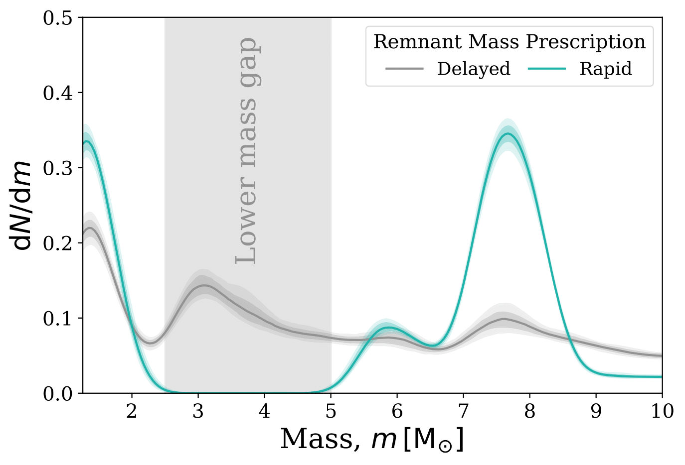
An interesting point to consider is whether LISA could be used to put constraints on the existence of the "lower mass gap". In the plot we show two curves that show the distribution of the masses of each component in all detectable sources (weighted by their detections rate, i.e. BHBHs are more important than NSNSs for the curve). Each curve uses a different remnant mass prescription, which is essentially a set of rules that define what sort of compact object a star becomes when it dies. The grey line uses a prescription that allows systems to be formed at any mass, whilst the blue line uses a prescription that forbids the formation of systems in the "lower mass gap" (from 2.5 to 5 solar masses).
“Over our binary physics variations, approximately 30-70% of LISA detections (or, in terms of detections, 15 to 156) will have at least one component in the lower mass gap
We see that if systems are formed with component masses in the gap, LISA will be able to detect them. For our fiducial model, 55% of systems that LISA will detect will have at least one component in the "lower mass gap". This fraction varies and we find over our binary physics variations, approximately 30-70% of LISA detections (or, in terms of detections, 15 to 156) will have at least one component in the lower mass gap. Overall, though the fraction in the gap varies, if DCOs are formed in the gap, LISA will detect them. The difficult comes in whether LISA will be able to measure the masses well enough to actually say that they are in the gap. It is therefore difficult to say whether LISA could potentially put constraints on the existence of a lower mass gap.
Can we identify the nature of every detected source?
So far we've talk about how many BHBHs, BHNSs and NSNSs LISA will detect and also what their properties will be. However, when the signal arrives in LISA we will, of course, not immediately know what type of DCO produced the signal. Let's talk about some methods we could use to identify the nature of the sources that we investigated.
How we do we know we're not seeing a double white dwarf?
The first important step to take is to distinguish the source from the double white dwarf (WDWD) background in LISA. WDWDs are by far the most prominent type of stellar-mass source in LISA so it could be easy to mistake one of the more massive DCOs for a WDWD. There are two main ways we could tell that a source is not a WDWD.
Mass: The maximum possible mass of a white dwarf is defined by the Chandrasekhar mass (about 1.2 solar masses). This means that if we can say with confidence that the total mass of a source is greater than twice the Chandrasekhar limit then we know it isn't a double white dwarf.
Eccentricity + sky position: It is expect that WDWDs that are formed within the disc of the galaxy will have little to no eccentricity. Therefore, if we can confidently state that a source is within the Galactic plane (given its sky position) and that it is eccentric, then it is not a WDWD.
If we combine these two methods and apply them to our fiducial model then we find that, in a 4-year mission, LISA will detect 37 BHBHs, 18 BHNSs and 5 NSNSs that can be confidently distinguished from WDWDs. This means that approximately half of all detections of more massive DCOs in LISA will be distinguishable from the double white dwarf background.
“Approximately half of all detections of more massive DCOs in LISA will be distinguishable from the double white dwarf background
What sort of double compact object is it then?
Well, this is where it gets difficult. For discriminating between NSNSs and the DCOs that contain a black hole, we can repeat a similar exercise to what we used for WDWDs. The maximum neutron star mass is around 2.5 solar masses and we can split the population to systems that don't contain any black holes and those that must contain at least one. For a 4-year mission, this would result in 16 BHBH, 7 BHNS and 4 NSNS detections where we can confidently state whether the system contains a black hole
Finally, for telling the difference between BHNSs and BHBHs it is difficult to say with certainty what the nature of the source is without an excellent measurement of the mass. One could possibly infer its nature from the source's frequency or eccentricity but this would only given an indication of which type is more likely rather than rule one out.
How do our results compare to similar studies?
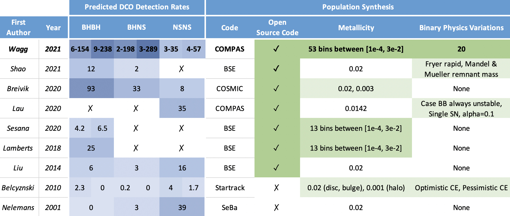
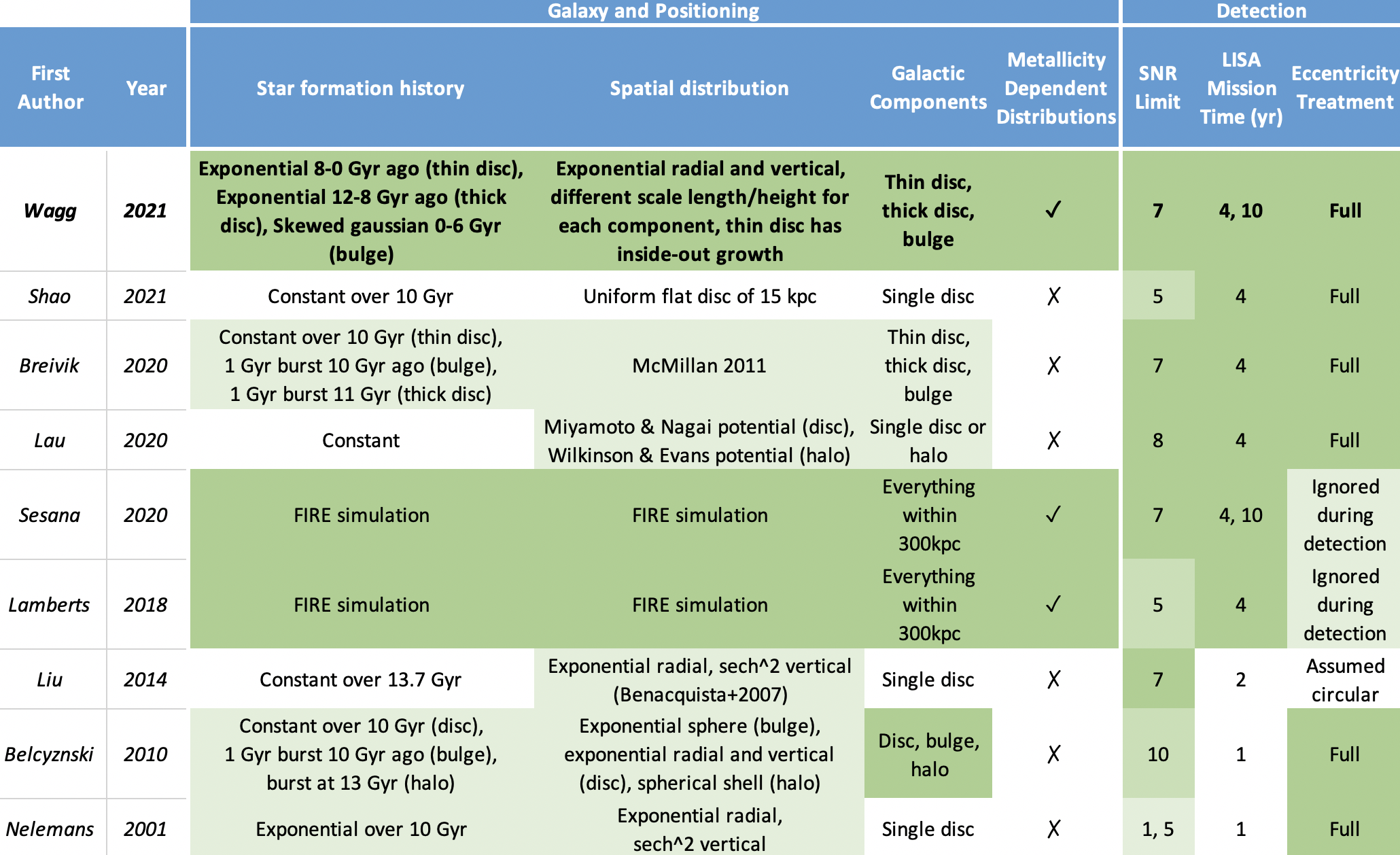
In Section 6 of the paper, we compare our results to similar studies that were conducted in the past. I recommend you read that section if you'd like to see what where we think the reasons for our differences come from. Below I include the table of comparisons that collated and you can examine the difference between the studies. For reference, in the later columns the darker the shade of green, the more reasonable/accurate we find the assumption.
Conclusions: you made it!
Click on each of the buttons below to read each of our main conclusions!